Tutorial 1: Parallelization Basics

This tutorial covers the fundamental concepts of parallelization in JAX, including device meshes, sharded arrays, and collective operations. We’ll build understanding step by step, starting with basic concepts and working towards practical implementations.

Learning objectives:

• Understand JAX’s device mesh and sharding concepts

• Learn about how matrices can be sharded across devices

• Learn about collective operations (AllGather, ReduceScatter, etc.)

• Implement basic parallel computations

Prerequisites:

• Basic familiarity with NumPy

• Understanding of matrix operations

• No prior knowledge of distributed computing required

0. Why JAX?

JAX is a high-performance numerical computing library that combines NumPy’s familiar API with the power of automatic differentiation and hardware acceleration on GPUs and TPUs. Developed by Google Research, JAX enables writing high-performance code that can run efficiently on a single device or scale across multiple devices.

We use JAX for this notebook (and in the MinText library) because of several reasons:

1. Beginner-friendly automatic parallelization using jax.jit

2. Ability to simulate multiple devices using "XLA_FLAGS"

3. Google Colab provides an 8 device runtime, v2-8 TPU, for free. This consists of 8x8 GB TPU cores which adds up to a total of 64 GB VRAM compute. So you can actually run distributed operations over 8 devices.

4. There are already several great pedagogical style libraries in Pytorch (such as HuggingFace Nanotron) which serve a similar purpose. The key concepts from these tutorials can often be directly translated to PyTorch.

1. Multi-Device Computation

Choose the v2-8 TPU runtime in Google Colab to run this notebook. Once you restart the and exploring the available devices.

# Install JAX if needed
# !pip install --upgrade jax jaxlib

# Uncomment this to simulate running the code on 8 CPU devices (use for local runs)
# import os
# os.environ["XLA_FLAGS"] = '--xla_force_host_platform_device_count=8' # Use 8 CPU devices

import jax
import jax.numpy as jnp
from jax.sharding import Mesh, NamedSharding, PartitionSpec as P
from jax.experimental import mesh_utils
from jax.experimental.shard_map import shard_map

from functools import partial
import numpy as np
import time
import matplotlib.pyplot as plt
from typing import Optional

# Check available devices
print(f"JAX version: {jax.__version__}")
print(f"Available devices: {jax.devices()}")
print(f"Device count: {jax.device_count()}")

JAX version: 0.5.2
Available devices: [TpuDevice(id=0, process_index=0, coords=(0,0,0), core_on_chip=0), TpuDevice(id=1, process_index=0, coords=(0,0,0), core_on_chip=1), TpuDevice(id=2, process_index=0, coords=(1,0,0), core_on_chip=0), TpuDevice(id=3, process_index=0, coords=(1,0,0), core_on_chip=1), TpuDevice(id=4, process_index=0, coords=(0,1,0), core_on_chip=0), TpuDevice(id=5, process_index=0, coords=(0,1,0), core_on_chip=1), TpuDevice(id=6, process_index=0, coords=(1,1,0), core_on_chip=0), TpuDevice(id=7, process_index=0, coords=(1,1,0), core_on_chip=1)]
Device count: 8

If you cannot access the v2-8 TPU from Google Colab (you timed out or are running this locally) restart this notebook and un-comment the os.environ["XLA_FLAGS"] = '--xla_force_host_platform_device_count=8' flag to simulate multiple devices on your CPU.

The output of the cell above should then change to look something like this:

Available devices: [CpuDevice(id=0), CpuDevice(id=1), CpuDevice(id=2), CpuDevice(id=3), CpuDevice(id=4), CpuDevice(id=5), CpuDevice(id=6), CpuDevice(id=7)]
Device count: 8

1.1 Creating a Device Mesh

JAX uses the concept of a device mesh to organize available devices. A device can be a CPU (or a CPU core), GPU, or TPU for JAX’s purpose. A mesh is a multi-dimensional array of devices that can be addressed along different axes. This allows us to partition our data and computation along different dimensions of the mesh.

devices = jax.devices()

# If you have multiple devices, you can create a 2D mesh
if len(devices) >= 4:
    mesh_2d = jax.make_mesh((2, 2), ('x', 'y'))
    print(f"2D Mesh: {mesh_2d}")
    print([d.id for d in mesh_2d.devices.flat])
else:
    print("Not enough devices for a 2D mesh demonstration")

2D Mesh: Mesh('x': 2, 'y': 2)
[0, 1, 2, 3]

2. Sharded Matrices

Sharded matrices are arrays that are split across multiple devices. JAX provides abstractions to create and operate on these distributed arrays efficiently.

2.1 Device Mesh and Partition Specifications

• Mesh: A logical arrangement of devices

• PartitionSpec (P): Specifies how to partition an array across mesh dimensions

• jax.device_put(): Places an array on a specific device or according to a sharding

Image Source: How To Scale Your Model

Let’s see how to create sharded arrays using JAX’s sharding API:

# Let's create a large matrix and shard it
matrix_size = 8192  # Adjust based on your device memory
matrix = jnp.ones((matrix_size, matrix_size))
print(f"Matrix shape: {matrix.shape}, Size in memory: {matrix.size * 4 / (1024**2):.2f} MB")

Matrix shape: (8192, 8192), Size in memory: 256.00 MB

# Define the partition spec - shard along the first dimension
partition_spec = P('x', 'y')

# Create a shardings object
from jax.sharding import NamedSharding
shardings = NamedSharding(mesh_2d, partition_spec)

# Create the sharded array
sharded_matrix = jax.device_put(x=matrix, device=shardings)

print(f"Sharded matrix type: {type(sharded_matrix)}")
print(f"Sharding spec: {shardings}")

jax.debug.visualize_array_sharding(sharded_matrix)

Sharded matrix type: <class 'jaxlib.xla_extension.ArrayImpl'>
Sharding spec: NamedSharding(mesh=Mesh('x': 2, 'y': 2), spec=PartitionSpec('x', 'y'), memory_kind=device)

                        
                        
   TPU 0       TPU 1    
                        
                        
                        
                        
                        
   TPU 2       TPU 3    
                        
                        
                        

2.2 Inspecting Sharded Matrices

We can inspect how the array is distributed across devices:

print("Global matrix shape", sharded_matrix.shape)

# Get the local arrays on each device
print("Shapes of Matrix Shards:")
for shard in sharded_matrix.addressable_shards:
  print(shard.device, shard.index, shard.data.shape)

Global matrix shape (8192, 8192)
Shapes of Matrix Shards:
TPU_0(process=0,(0,0,0,0)) (slice(0, 4096, None), slice(0, 4096, None)) (4096, 4096)
TPU_1(process=0,(0,0,0,1)) (slice(0, 4096, None), slice(4096, 8192, None)) (4096, 4096)
TPU_2(process=0,(1,0,0,0)) (slice(4096, 8192, None), slice(0, 4096, None)) (4096, 4096)
TPU_3(process=0,(1,0,0,1)) (slice(4096, 8192, None), slice(4096, 8192, None)) (4096, 4096)

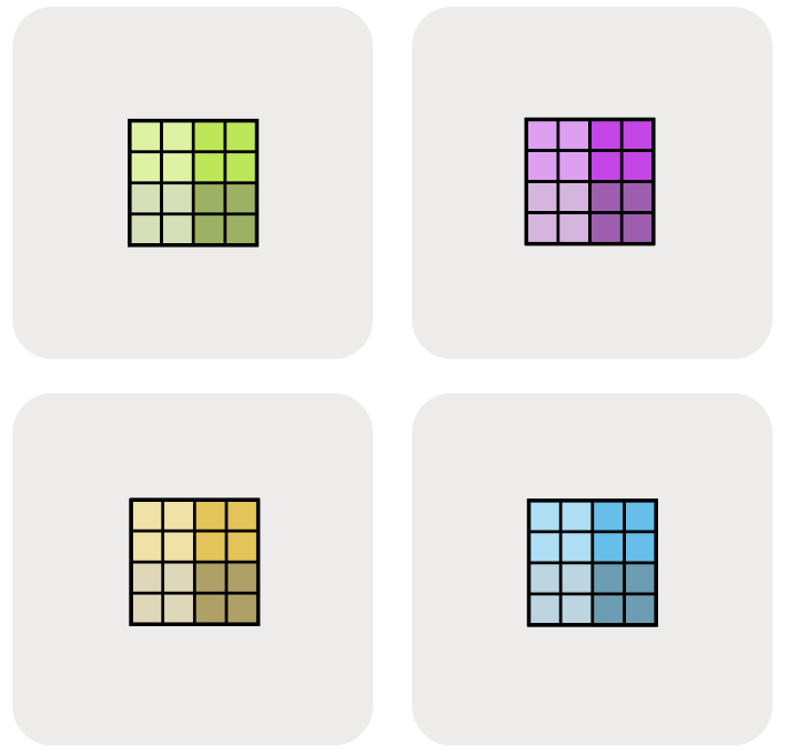
Image Source: How To Scale Your Model

2.3 Performance Benefits

Let’s compare the performance of element-wise operations on sharded vs. non-sharded matrices (we will matrix-level operations in a bit)

# `matrix` is present on a single device
%timeit -n 5 -r 5 jnp.sin(matrix).block_until_ready()

The slowest run took 10.40 times longer than the fastest. This could mean that an intermediate result is being cached.
27.9 ms ± 36.2 ms per loop (mean ± std. dev. of 5 runs, 5 loops each)

# `sharded_matrix` is distributed across 4 devices
%timeit -n 5 -r 5 jnp.sin(sharded_matrix).block_until_ready()

The slowest run took 29.52 times longer than the fastest. This could mean that an intermediate result is being cached.
21.4 ms ± 36.2 ms per loop (mean ± std. dev. of 5 runs, 5 loops each)

2.4 Sharding Strategies

Each axis of the matrix can be sharded across each possible axis in the device mesh. This gives rise to a combinatorial number of possible shardings.

# A small helper function to define a sharding mesh
default_mesh = jax.make_mesh((2, 2), ('x', 'y'))

def mesh_sharding(
    pspec: P, mesh: Optional[Mesh] = None,
  ) -> NamedSharding:
  if mesh is None:
    mesh = default_mesh
  return NamedSharding(mesh, pspec)

# Shard first axis of matrix along mesh axis 'x', second axis of matrix along mesh axis 'y'
ix_jy_sharding = jax.device_put(matrix, mesh_sharding(P('x', 'y')))
jax.debug.visualize_array_sharding(ix_jy_sharding)

                        
                        
   TPU 0       TPU 1    
                        
                        
                        
                        
                        
   TPU 2       TPU 3    
                        
                        
                        

# Shard first axis of matrix along mesh axis 'y', second axis of matrix along mesh axis 'x'
iy_jx_sharding = jax.device_put(matrix, mesh_sharding(P('x', 'y')))
jax.debug.visualize_array_sharding(iy_jx_sharding)

                        
                        
   TPU 0       TPU 2    
                        
                        
                        
                        
                        
   TPU 1       TPU 3    
                        
                        
                        

# Shard first axis of matrix along mesh axis 'x', replicate second axis of matrix along each shard
ix_j_sharding = jax.device_put(matrix, mesh_sharding(P('x', None)))
jax.debug.visualize_array_sharding(ix_j_sharding, use_color=False)

┌───────────────────────┐
│                       │
│        TPU 0,1        │
│                       │
│                       │
├───────────────────────┤
│                       │
│        TPU 2,3        │
│                       │
│                       │
└───────────────────────┘

# Partition second axis of x over second mesh axis 'y', replicate first axis of matrix along each shard
i_jy_shard = jax.device_put(matrix, mesh_sharding(P(None, 'y')))
jax.debug.visualize_array_sharding(i_jy_shard, use_color=False)

┌──────────┬──────────┐
│          │          │
│          │          │
│          │          │
│          │          │
│ TPU 0,2  │ TPU 1,3  │
│          │          │
│          │          │
│          │          │
│          │          │
└──────────┴──────────┘

For a 2D matrix being sharded along a 2D device mesh, here are all the possible sharding strategies

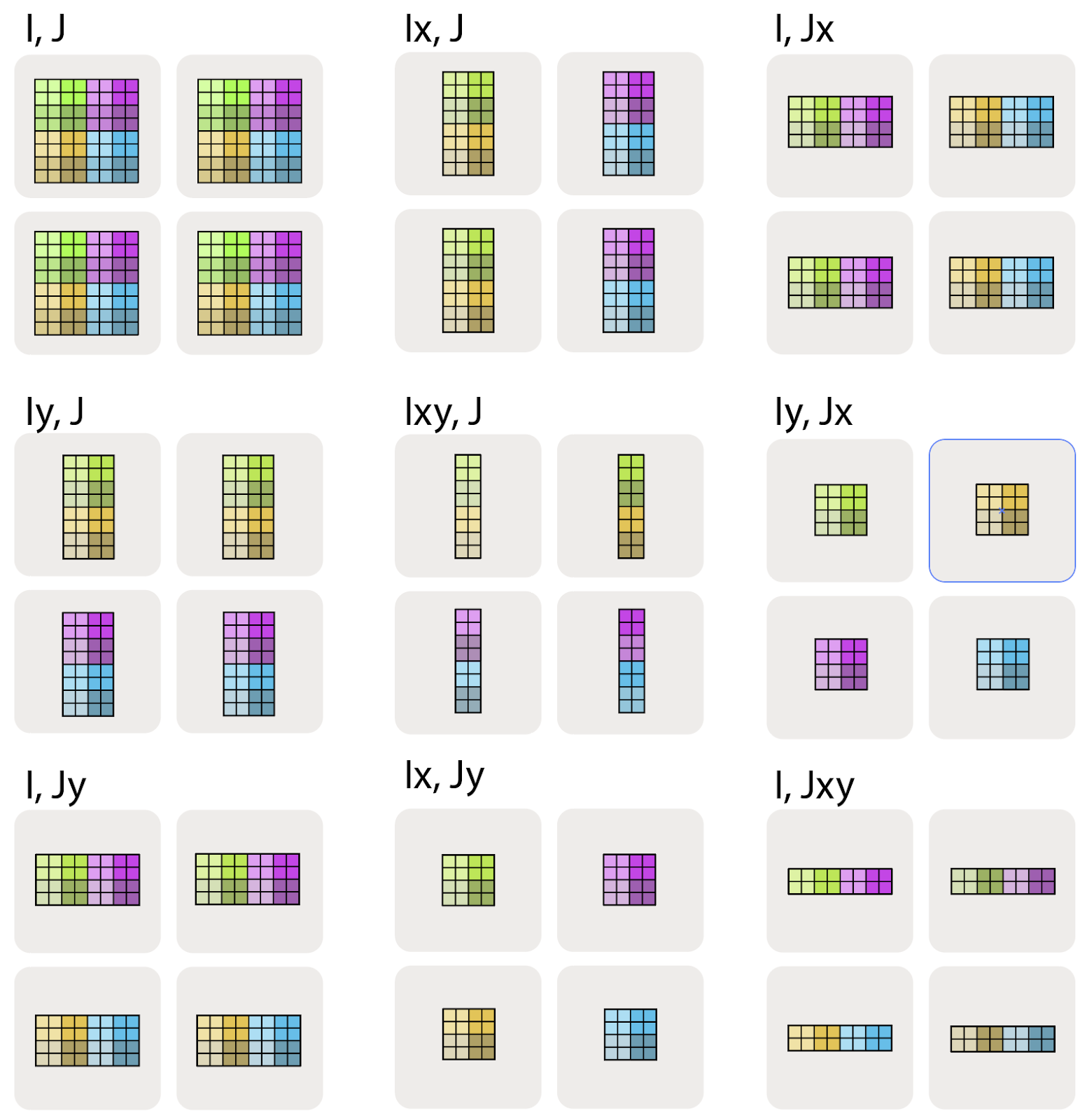
Image Source: How To Scale Your Model

2.5 Choosing the Right Sharding Strategy

As we discuss collectives (next section) and different parallelism strategies in (next tutorials), we will slowly do a deeper dive into how to chose sharding strategies based on your use case.

3. Collective Operations

Collective operations are essential for distributed algorithms where devices need to share or aggregate information. In deep learning, these are utilized in performing computations with sharded arrays.

3.1 Matrix Operations With Sharded Arrays

If we want to perform matrix operations on sharded arrays, we need to think through some overheads involved in moving data between devices.

In deep learning, these two operations are often used:

• Element-wise operations (e.g. ReLU): Operations that can be performed independently on each element of the array. These operations can be performed in parallel across aray shards without needing to communicate between them.

• Matrix-multiplication (e.g. Linear Layer, Attention etc): A more complex operation that requires communication between devices to compute the result. This is where collective operations come into play.

3.1.1 Block Matrix Multiplication

We can think of a matrix as being composed of smaller blocks, which can be processed independently.

\begin{equation} \begin{pmatrix} a_{00} & a_{01} & a_{02} & a_{03} \\ a_{10} & a_{11} & a_{12} & a_{13} \\ a_{20} & a_{21} & a_{22} & a_{23} \\ a_{30} & a_{31} & a_{32} & a_{33} \end{pmatrix} = \left( \begin{matrix} \begin{bmatrix} a_{00} & a_{01} \\ a_{10} & a_{11} \end{bmatrix} \\ \begin{bmatrix} a_{20} & a_{21} \\ a_{30} & a_{31} \end{bmatrix} \end{matrix} \begin{matrix} \begin{bmatrix} a_{02} & a_{03} \\ a_{12} & a_{13} \end{bmatrix} \\ \begin{bmatrix} a_{22} & a_{23} \\ a_{32} & a_{33} \end{bmatrix} \end{matrix} \right) = \begin{pmatrix} \mathbf{A_{00}} & \mathbf{A_{01}} \\ \mathbf{A_{10}} & \mathbf{A_{11}} \end{pmatrix} \end{equation}

Matrix multiplication carries this nice property that the product of two matrices can be written in terms of block matmuls.

\begin{equation} \begin{pmatrix} A_{00} & A_{01} \\ A_{10} & A_{11} \end{pmatrix} \cdot \begin{pmatrix} B_{00} & B_{01} \\ B_{10} & B_{11} \end{pmatrix} = \begin{pmatrix} A_{00}B_{00} + A_{01}B_{10} & A_{00}B_{01} + A_{01}B_{11} \\ A_{10}B_{00} + A_{11}B_{10} & A_{10}B_{01} + A_{11}B_{11} \end{pmatrix} \end{equation}

So we can compute distributed matrix multiplication by computing the block matmuls in parallel. The question is what communication is required to compute the final result, when to do it, and how expensive it is to perform.

# Create a 2x2 mesh with 4 devices to visualize matmul examples
mesh_2x2 = jax.make_mesh((2, 2), ('x', 'y'))

3.2 Case 1: No Sharded Contracting Dimension

Consider the matrix multiplication of two sharded matrices \(\mathbf{A}[I_X, J]\) and \(\mathbf{B}[J, K_Y]\). Note that the contracting dimension \(J\) is not sharded. Thus we have:

\[\mathbf{A}[I_X, J] \cdot \mathbf{B}[J, K_Y] \rightarrow \mathbf{C}[I_X, K_Y]\]

Example: Case 1 - No Sharded Contracting Dimension

Let’s demonstrate this with 4x4 matrices on a 2x2 mesh where the contracting dimension is not sharded:

# Case 1: No sharded contracting dimension
# A[I_X, J] @ B[J, K_Y] -> C[I_X, K_Y]

# Create two small 4x4 matrices
key = jax.random.PRNGKey(42)
A = jax.random.uniform(key, (4, 4))
B = jax.random.uniform(key, (4, 4)) + 1

# Shard A along first dimension (rows) on X axis, B along second dimension (columns) on Y axis
A_sharded = jax.device_put(A, NamedSharding(mesh_2x2, P('x', None)))
B_sharded = jax.device_put(B, NamedSharding(mesh_2x2, P(None, 'y')))

print("Matrix A sharding (rows split along X):")
jax.debug.visualize_array_sharding(A_sharded)
print("\nMatrix B sharding (columns split along Y):")
jax.debug.visualize_array_sharding(B_sharded)

# Direct multiplication works without any collective operations
C = A_sharded @ B_sharded
print("\nResult C sharding (both dimensions sharded):")
jax.debug.visualize_array_sharding(C)

# Verify the result
C_expected = A @ B
print(f"\nCorrect result: {jnp.allclose(C, C_expected)}")
print(f"C shape: {C.shape}")

Matrix A sharding (rows split along X):

                         
                         
         TPU 0,1         
                         
                         
                         
                         
                         
         TPU 2,3         
                         
                         
                         

Matrix B sharding (columns split along Y):

                        
                        
                        
                        
                        
  TPU 0,2     TPU 1,3   
                        
                        
                        
                        
                        

Result C sharding (both dimensions sharded):

                        
                        
   TPU 0       TPU 1    
                        
                        
                        
                        
                        
   TPU 2       TPU 3    
                        
                        
                        

Correct result: True
C shape: (4, 4)

We can multiply each local shard without any communication between devices. Each device computes its local shard of the result matrix \(\mathbf{C}\) independently. Each of the following possible sharded matrix multiplications can be performed without any communication:

\begin{align*} \mathbf{A}[I, J] \cdot \mathbf{B}[J, K] \rightarrow &\ \mathbf{C}[I, K] \\ \mathbf{A}[I_X, J] \cdot \mathbf{B}[J, K] \rightarrow &\ \mathbf{C}[I_X, K]\\ \mathbf{A}[I, J] \cdot \mathbf{B}[J, K_Y] \rightarrow &\ \mathbf{C}[I, K_Y]\\ \mathbf{A}[I_X, J] \cdot \mathbf{B}[J, K_Y] \rightarrow &\ \mathbf{C}[I_X, K_Y] \end{align*}

3.3 Case 2 (All-Gather): One matrix has a sharded contracting dimension

Consider the case of a distributed matrix multiplication where one of the matrices has a sharded contracting dimension. For example,

\[\mathbf{A}[I, J_X] \cdot \mathbf{B}[J, K] \rightarrow \mathbf{C}[I, K]\]

Now, we cannot directly multiply the local shards of \(\mathbf{A}\) and \(\mathbf{B}\) without communication. Each device needs to gather the shards of \(\mathbf{B}\) across all devices to compute its local shard of \(\mathbf{C}\). This is done using an all-gather operation.

# Case 2: Show why direct multiplication fails
# A[I, J_X] @ B[J, K] - contracting dimension J is sharded in A

# Create matrices
A = jnp.arange(16).reshape(4, 4).astype(jnp.float32)
B = jnp.arange(16, 32).reshape(4, 4).astype(jnp.float32)

# Shard A's columns (contracting dimension) along X axis
A_sharded = jax.device_put(A, NamedSharding(mesh_2x2, P(None, 'x')))
B_unsharded = B  # B is replicated

print("Matrix A sharding (columns split along X - contracting dimension):")
jax.debug.visualize_array_sharding(A_sharded, use_color=False)
print("\nMatrix B (replicated on all devices):")
jax.debug.visualize_array_sharding(B_unsharded, use_color=False)

# Show what each device sees locally
print("\nWhat each device sees locally:")
for shard in A_sharded.addressable_shards[:3:2]:  # Show each group of devices
    print(f"\nDevice {shard.device.id} has A columns {shard.index[1]}:")
    print(shard.data)
    print("But needs ALL columns of A to multiply with B!")

# This would fail or give incorrect results if done locally
print("\n⚠️  Cannot multiply directly - each device only has partial columns of A")

Matrix A sharding (columns split along X - contracting dimension):

┌──────────┬──────────┐
│          │          │
│          │          │
│          │          │
│          │          │
│ TPU 0,1  │ TPU 2,3  │
│          │          │
│          │          │
│          │          │
│          │          │
└──────────┴──────────┘

Matrix B (replicated on all devices):

┌───────────────────────┐
│                       │
│                       │
│                       │
│                       │
│         TPU 0         │
│                       │
│                       │
│                       │
│                       │
└───────────────────────┘

What each device sees locally:

Device 0 has A columns slice(0, 2, None):
[[ 0.  1.]
 [ 4.  5.]
 [ 8.  9.]
 [12. 13.]]
But needs ALL columns of A to multiply with B!

Device 2 has A columns slice(2, 4, None):
[[ 2.  3.]
 [ 6.  7.]
 [10. 11.]
 [14. 15.]]
But needs ALL columns of A to multiply with B!

⚠️  Cannot multiply directly - each device only has partial columns of A

All Gather is a collective operation that gathers data from all devices and distributes it to all devices. In this case, each device gathers the shards of an array across all devices and gets a fully replicated array.

Here is a simple example of how to perform an All-Gather operation in JAX:

Image Source: JAX documentation

mesh1d = Mesh(jax.devices()[:4], ('i',))

@partial(shard_map, mesh=mesh1d, in_specs=P('i'), out_specs=P('i'))
def all_gather(x_block):
  print('BEFORE:', x_block)
  y_block = jax.lax.all_gather(x_block, 'i', tiled=True)
  print('AFTER:', y_block)
  return y_block

x = jnp.array([3, 9, 5, 2])
y = all_gather(x)
print('FINAL RESULT:', y)

BEFORE: On TPU_0(process=0,(0,0,0,0)) at mesh coordinates (i,) = (0,):
[3]

On TPU_1(process=0,(0,0,0,1)) at mesh coordinates (i,) = (1,):
[9]

On TPU_2(process=0,(1,0,0,0)) at mesh coordinates (i,) = (2,):
[5]

On TPU_3(process=0,(1,0,0,1)) at mesh coordinates (i,) = (3,):
[2]

AFTER: On TPU_0(process=0,(0,0,0,0)) at mesh coordinates (i,) = (0,):
[3 9 5 2]

On TPU_1(process=0,(0,0,0,1)) at mesh coordinates (i,) = (1,):
[3 9 5 2]

On TPU_2(process=0,(1,0,0,0)) at mesh coordinates (i,) = (2,):
[3 9 5 2]

On TPU_3(process=0,(1,0,0,1)) at mesh coordinates (i,) = (3,):
[3 9 5 2]

FINAL RESULT: [3 9 5 2 3 9 5 2 3 9 5 2 3 9 5 2]

To perform a matrix multiplication using the AllGather operation, we can follow these steps:

1. AllGather the first matrix across all devices.

   \[\textbf{AllGather}_X[I, J_X] \rightarrow \mathbf{A}[I, J]\]

2. Multiply the gathered matrix with the second matrix.

   \[\mathbf{A}[I, J] \cdot \mathbf{B}[J, K] \rightarrow \mathbf{C}[I, K]\]

Example: Case 2 - One Matrix has Sharded Contracting Dimension

# Case 2: Solution using All-Gather
# Step 1: All-gather A to reconstruct full matrix on each device
# Step 2: Multiply with B

@partial(shard_map, mesh=mesh_2x2,
         in_specs=(P(None, 'X'), P(None, None)),
         out_specs=P(None, None),
         check_rep=False)
def matmul_with_allgather(A_shard, B_shard):
    print(f"Before all-gather, A_shard shape: {A_shard.shape}")

    # All-gather along the X axis to get full A matrix
    A_full = jax.lax.all_gather(A_shard, 'X', axis=1, tiled=True)
    print(f"After all-gather, A_full shape: {A_full.shape}")

    # Now we can multiply
    C = A_full @ B_shard
    return C

# Execute the multiplication with all-gather
try:
  C = matmul_with_allgather(A_sharded, B_unsharded)
except Exception as e:
  print("An error occurred:", e)

print("\nResult C (replicated on all devices):")
jax.debug.visualize_array_sharding(C)

# Verify correctness
C_expected = A @ B
print(f"\nCorrect result: {jnp.allclose(C, C_expected)}")
print(f"Result shape: {C.shape}")
print(f"\nFirst few elements of result:\n{C[:2, :2]}")

Before all-gather, A_shard shape: (4, 2)
After all-gather, A_full shape: (4, 4)

Result C (replicated on all devices):

                         
                         
                         
                         
                         
       TPU 0,1,2,3       
                         
                         
                         
                         
                         

Correct result: True
Result shape: (4, 4)

First few elements of result:
[[152. 158.]
 [504. 526.]]

3.3.1 How is an all-gather performed?

Image Source: How To Scale Your Model

3.4 Case 3 (All-Reduce): Both Matrices have sharded contracting dimensions

Consider the case where both matrices to be multiplied are sharded on their contracting dimensions, along the same mesh axes.

\[\textbf{A}[I, J_X] \cdot \textbf{B}[J_X, K] \rightarrow C[I, K]\]

In this case, we can multiply the local shards of the matrices, however each shard will only contain a partial result.

\[\textbf{A}[I, J_X] \cdot_\text{LOCAL} \textbf{B}[J_X, K] \rightarrow C[I, K] \{\ U_X \}\]

The notation \(\{\ U_X \}\) here refers to the fact that the matrix \(C\) is unreduced along the mesh axis \(X\).

# Case 3: Show why we need all-reduce
# A[I, J_X] @ B[J_X, K] - contracting dimension J is sharded in both

# Create matrices
A = jnp.arange(16).reshape(4, 4).astype(jnp.float32)
B = jnp.arange(16, 32).reshape(4, 4).astype(jnp.float32)

# Shard contracting dimensions along X axis
A_sharded = jax.device_put(A, NamedSharding(mesh_2x2, P(None, 'x')))
B_sharded = jax.device_put(B, NamedSharding(mesh_2x2, P('x', None)))

print("Matrix A sharding (columns split along X):")
jax.debug.visualize_array_sharding(A_sharded, use_color=False)
print("\nMatrix B sharding (rows split along X):")
jax.debug.visualize_array_sharding(B_sharded, use_color=False)

# Show what happens with local multiplication
print("\nLocal multiplication on each device:")
print("Device 0: A[:, 0:2] @ B[0:2, :] = partial result")
print("Device 1: A[:, 2:4] @ B[2:4, :] = partial result")
print("\nEach device computes only PART of the final result!")
print("Need to SUM all partial results to get the correct answer")

Matrix A sharding (columns split along X):

┌──────────┬──────────┐
│          │          │
│          │          │
│          │          │
│          │          │
│ TPU 0,1  │ TPU 2,3  │
│          │          │
│          │          │
│          │          │
│          │          │
└──────────┴──────────┘

Matrix B sharding (rows split along X):

┌───────────────────────┐
│                       │
│        TPU 0,1        │
│                       │
│                       │
├───────────────────────┤
│                       │
│        TPU 2,3        │
│                       │
│                       │
└───────────────────────┘

Local multiplication on each device:
Device 0: A[:, 0:2] @ B[0:2, :] = partial result
Device 1: A[:, 2:4] @ B[2:4, :] = partial result

Each device computes only PART of the final result!
Need to SUM all partial results to get the correct answer

To obtain the final result, we need to perform an All-Reduce operation on the shards of \(C\). Since the all-reduce sum operation is very common, jax provides the jax.lax.psum function to perform this operation efficiently.

@partial(shard_map, mesh=mesh1d, in_specs=P('i'), out_specs=P(None))
def psum(x_block):
  print('BEFORE:\n', x_block)
  y_block = jax.lax.psum(x_block, 'i')
  print('AFTER:\n', y_block)
  return y_block

x = jnp.array([3, 1, 4, 1, 5, 9, 2, 6, 5, 3, 5, 8, 9, 7, 1, 2])
y = psum(x)
print('FINAL RESULT:\n', y)

BEFORE:
 On TPU_0(process=0,(0,0,0,0)) at mesh coordinates (i,) = (0,):
[3 1 4 1]

On TPU_1(process=0,(0,0,0,1)) at mesh coordinates (i,) = (1,):
[5 9 2 6]

On TPU_2(process=0,(1,0,0,0)) at mesh coordinates (i,) = (2,):
[5 3 5 8]

On TPU_3(process=0,(1,0,0,1)) at mesh coordinates (i,) = (3,):
[9 7 1 2]

AFTER:
 On TPU_0(process=0,(0,0,0,0)) at mesh coordinates (i,) = (0,):
[22 20 12 17]

On TPU_1(process=0,(0,0,0,1)) at mesh coordinates (i,) = (1,):
[22 20 12 17]

On TPU_2(process=0,(1,0,0,0)) at mesh coordinates (i,) = (2,):
[22 20 12 17]

On TPU_3(process=0,(1,0,0,1)) at mesh coordinates (i,) = (3,):
[22 20 12 17]

FINAL RESULT:
 [22 20 12 17]

Example: Case 3 - Both Matrices have Sharded Contracting Dimensions

When both matrices have their contracting dimensions sharded along the same axis, we can multiply locally but need to sum the partial results:

In order to perform the matrix multiplication \(C = A \cdot B\) using the AllReduce operation, we can break down the process into two main steps.

1. Local Matrix Multiplication of input matrix shards on each device.

   \[A[I, J_X] \cdot_\text{LOCAL} B[J_X, K] \rightarrow C[I, K] \{ U_X \}\]

2. AllReduce the partial results across all devices.

   \[\textbf{AllReduce}_X C[I, K] \{ U_X \} \rightarrow C[I, K]\]

# Case 3: Solution using All-Reduce (psum)
# Step 1: Local matrix multiplication
# Step 2: All-reduce (sum) the partial results

@partial(shard_map, mesh=mesh_2x2,
         in_specs=(P(None, 'x'), P('x', None)),
         out_specs=P(None, None))
def matmul_with_allreduce(A_shard, B_shard):
    print(f"Local shard shapes: A={A_shard.shape}, B={B_shard.shape}")

    # Step 1: Local multiplication (each device computes partial result)
    C_partial = A_shard @ B_shard
    print(f"Partial result shape: {C_partial.shape}")

    # Step 2: All-reduce (sum) across X axis
    C_full = jax.lax.psum(C_partial, 'x')
    print(f"After all-reduce shape: {C_full.shape}")

    return C_full

# Execute the multiplication with all-reduce
C = matmul_with_allreduce(A_sharded, B_sharded)

print("\nResult C (replicated on all devices after all-reduce):")
jax.debug.visualize_array_sharding(C)

# Verify correctness
C_expected = A @ B
print(f"\nCorrect result: {jnp.allclose(C, C_expected)}")
print(f"Result shape: {C.shape}")

# Show the computation breakdown
print("\nComputation breakdown:")
print(f"A[:, 0:2] @ B[0:2, :] + A[:, 2:4] @ B[2:4, :] = Full result")
print(f"\nFirst few elements of result:\n{C[:2, :2]}")

Local shard shapes: A=(4, 2), B=(2, 4)
Partial result shape: (4, 4)
After all-reduce shape: (4, 4)

Result C (replicated on all devices after all-reduce):

                         
                         
                         
                         
                         
       TPU 0,1,2,3       
                         
                         
                         
                         
                         

Correct result: True
Result shape: (4, 4)

Computation breakdown:
A[:, 0:2] @ B[0:2, :] + A[:, 2:4] @ B[2:4, :] = Full result

First few elements of result:
[[152. 158.]
 [504. 526.]]

3.4.1 All-Reduce as ReduceScatter + AllGather

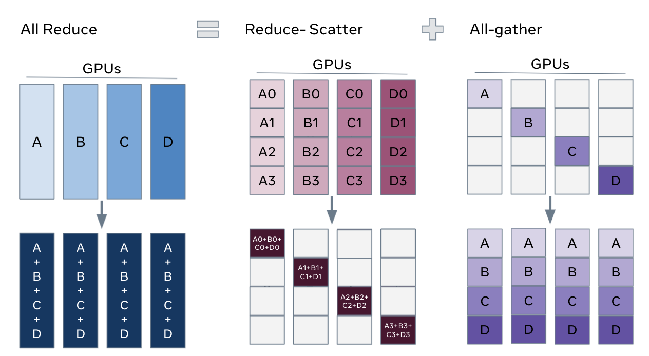
We can express AllReduce as two different collectives, a Reduce Scatter followed by AllGather. A Reduce Scatter operation is visualized below

@partial(shard_map, mesh=mesh1d, in_specs=P('i'), out_specs=P('i'))
def scatter_gather_sum(x_block):
  print('BEFORE:\n', x_block)
  y_block = jax.lax.psum_scatter(x_block, 'i', tiled=True)
  print('AFTER:\n', y_block)
  return y_block

x = jnp.array([3, 1, 4, 1, 5, 9, 2, 6, 5, 3, 5, 8, 9, 7, 1, 2])
y = scatter_gather_sum(x)
print('FINAL RESULT:\n', y)

BEFORE:
 On TPU_0(process=0,(0,0,0,0)) at mesh coordinates (i,) = (0,):
[3 1 4 1]

On TPU_1(process=0,(0,0,0,1)) at mesh coordinates (i,) = (1,):
[5 9 2 6]

On TPU_2(process=0,(1,0,0,0)) at mesh coordinates (i,) = (2,):
[5 3 5 8]

On TPU_3(process=0,(1,0,0,1)) at mesh coordinates (i,) = (3,):
[9 7 1 2]

AFTER:
 On TPU_0(process=0,(0,0,0,0)) at mesh coordinates (i,) = (0,):
[22]

On TPU_1(process=0,(0,0,0,1)) at mesh coordinates (i,) = (1,):
[20]

On TPU_2(process=0,(1,0,0,0)) at mesh coordinates (i,) = (2,):
[12]

On TPU_3(process=0,(1,0,0,1)) at mesh coordinates (i,) = (3,):
[17]

FINAL RESULT:
 [22 20 12 17]

3.5 Case 4 (All-Gather): Both Matrices have non-contracting dimensions sharded along the same mesh axes

Whenever we shard a tensor, each mesh dimension can appear AT MOST ONCE. Consider the case where both matrices to be multiplied are sharded on their non-contracting dimensions, along the same mesh axes.

\[\textbf{A}[I_X, J] \cdot \textbf{B}[J, K_X] \rightarrow C[I_X, K_X]\]

Such a sharding is not allowed, as there is not enough information along each shards to reconstruct the full matrix. In this case, we need to change the sharding of at least one of the matrices before multiplication.

# Case 4: Show the problem with both non-contracting dimensions sharded
# A[I_X, J] @ B[J, K_X] - trying to get C[I_X, K_X] is problematic

# Create matrices
A = jnp.arange(16).reshape(4, 4).astype(jnp.float32)
B = jnp.arange(16, 32).reshape(4, 4).astype(jnp.float32)

# Shard non-contracting dimensions on same axis X
A_sharded = jax.device_put(A, NamedSharding(mesh_2x2, P('x', None)))
B_sharded = jax.device_put(B, NamedSharding(mesh_2x2, P(None, 'x')))

print("Matrix A sharding (rows split along X):")
jax.debug.visualize_array_sharding(A_sharded, use_color=False)
print("\nMatrix B sharding (columns split along X):")
jax.debug.visualize_array_sharding(B_sharded, use_color=False)

print("\n⚠️  Problem: Each device needs data from OTHER devices!")
print("Device 0 has: A[0:2, :] and B[:, 0:2]")
print("But to compute C[0:2, 0:2], it needs ALL of A[0:2, :] @ ALL of B!")
print("Similarly, to compute C[0:2, 2:4], it needs A[0:2, :] @ B[:, 2:4]")
print("\nCannot compute the result without resharding!")

Matrix A sharding (rows split along X):

┌───────────────────────┐
│                       │
│        TPU 0,1        │
│                       │
│                       │
├───────────────────────┤
│                       │
│        TPU 2,3        │
│                       │
│                       │
└───────────────────────┘

Matrix B sharding (columns split along X):

┌──────────┬──────────┐
│          │          │
│          │          │
│          │          │
│          │          │
│ TPU 0,1  │ TPU 2,3  │
│          │          │
│          │          │
│          │          │
│          │          │
└──────────┴──────────┘

⚠️  Problem: Each device needs data from OTHER devices!
Device 0 has: A[0:2, :] and B[:, 0:2]
But to compute C[0:2, 0:2], it needs ALL of A[0:2, :] @ ALL of B!
Similarly, to compute C[0:2, 2:4], it needs A[0:2, :] @ B[:, 2:4]

Cannot compute the result without resharding!

We have two options:

1. All-Gather the sharding dimension of matrix A to have the non-contracting dimension unsharded.

   \[\begin{split}\begin{align*} \textbf{AllGather}_X A[I_X, J] \rightarrow &\ A[I, J] \\ A[I, J] \cdot B[J, K_X] \rightarrow &\ C[I, K_X] \end{align*}\end{split}\]

2. All-Gather the sharding dimension of matrix B to have the non-contracting dimension unsharded.

   \[\begin{split}\begin{align*} \textbf{AllGather}_X B[J, K_X] \rightarrow &\ B[J, K] \\ A[I_X, J] \cdot B[J, K] \rightarrow &\ C[I_X, K] \end{align*}\end{split}\]

Example: Both Matrices have non-contracting dimensions sharded along the same mesh axes

# Case 4: Solution - All-gather one of the matrices
# Option 1: All-gather B to remove column sharding

@partial(shard_map, mesh=mesh_2x2,
         in_specs=(P('x', None), P(None, 'x')),
         out_specs=P('x', None))
def matmul_case4_allgather_B(A_shard, B_shard):
    print(f"Before all-gather: A={A_shard.shape}, B={B_shard.shape}")

    # All-gather B along X axis to get full B on each device
    B_full = jax.lax.all_gather(B_shard, 'x', axis=1, tiled=True)
    print(f"After all-gather B: B_full={B_full.shape}")

    # Now multiply: each device computes its rows of C
    C_shard = A_shard @ B_full
    print(f"Result shape: {C_shard.shape}")

    return C_shard

# Execute the multiplication
C = matmul_case4_allgather_B(A_sharded, B_sharded)

print("\nResult C sharding (rows split along X):")
jax.debug.visualize_array_sharding(C, use_color=False)

# Verify correctness
C_expected = A @ B
print(f"\nCorrect result: {jnp.allclose(C, C_expected)}")
print(f"Result shape: {C.shape}")

# Alternative: All-gather A instead
print("\n--- Alternative: All-gather A instead of B ---")

@partial(shard_map, mesh=mesh_2x2,
         in_specs=(P('x', None), P(None, 'x')),
         out_specs=P(None, 'x'))
def matmul_case4_allgather_A(A_shard, B_shard):
    # All-gather A along X axis
    A_full = jax.lax.all_gather(A_shard, 'x', axis=0, tiled=True)
    # Multiply to get column-sharded result
    C_shard = A_full @ B_shard
    return C_shard

C_alt = matmul_case4_allgather_A(A_sharded, B_sharded)
print("Result with A gathered (columns split along X):")
jax.debug.visualize_array_sharding(C_alt, use_color=False)
print(f"Also correct: {jnp.allclose(C_alt, C_expected)}")

Before all-gather: A=(2, 4), B=(4, 2)
After all-gather B: B_full=(4, 4)
Result shape: (2, 4)

Result C sharding (rows split along X):

┌───────────────────────┐
│                       │
│        TPU 0,1        │
│                       │
│                       │
├───────────────────────┤
│                       │
│        TPU 2,3        │
│                       │
│                       │
└───────────────────────┘

Correct result: True
Result shape: (4, 4)

--- Alternative: All-gather A instead of B ---
Result with A gathered (columns split along X):

┌──────────┬──────────┐
│          │          │
│          │          │
│          │          │
│          │          │
│ TPU 0,1  │ TPU 2,3  │
│          │          │
│          │          │
│          │          │
│          │          │
└──────────┴──────────┘

Also correct: True

3.6 Other Collectives

3.6.2 All-to-All

All-to-all exchanges slices of data between all devices. This is useful for operations like matrix transposition or redistributing data with a different sharding. It is not used in the three parallelism strategies we will discuss, but is used in other parallelism (mentioned in tutorial 4).

@partial(shard_map, mesh=mesh1d, in_specs=P('i'), out_specs=P('i'))
def all_to_all(x_block):
  print('BEFORE:\n', x_block)
  y_block = jax.lax.all_to_all(x_block, 'i', split_axis=0, concat_axis=0,
                               tiled=True)
  print('AFTER:\n', y_block)
  return y_block

x = jnp.array([3, 1, 4, 1, 5, 9, 2, 6, 5, 3, 5, 8, 9, 7, 1, 2])
y = all_to_all(x)
print('FINAL RESULT:\n', y)

BEFORE:
 On TPU_0(process=0,(0,0,0,0)) at mesh coordinates (i,) = (0,):
[3 1 4 1]

On TPU_1(process=0,(0,0,0,1)) at mesh coordinates (i,) = (1,):
[5 9 2 6]

On TPU_2(process=0,(1,0,0,0)) at mesh coordinates (i,) = (2,):
[5 3 5 8]

On TPU_3(process=0,(1,0,0,1)) at mesh coordinates (i,) = (3,):
[9 7 1 2]

AFTER:
 On TPU_0(process=0,(0,0,0,0)) at mesh coordinates (i,) = (0,):
[3 5 5 9]

On TPU_1(process=0,(0,0,0,1)) at mesh coordinates (i,) = (1,):
[1 9 3 7]

On TPU_2(process=0,(1,0,0,0)) at mesh coordinates (i,) = (2,):
[4 2 5 1]

On TPU_3(process=0,(1,0,0,1)) at mesh coordinates (i,) = (3,):
[1 6 8 2]

FINAL RESULT:
 [3 5 5 9 1 9 3 7 4 2 5 1 1 6 8 2]

4. Notes on JAX Sharding

Mode	View?	Explicit sharding?	Explicit Collectives?
Auto	Global	❌	❌
Explicit	Global	✅	❌
Manual	Per-device	✅	✅

JAX provides three levels of granularity for sharding and parallelism, and they are summarized in the table above. For the purpose of these tutorials, we will focus mostly on the Auto and Explicit mode, which allows us to at most specify the sharding of arrays and not have to worry about collectives. The examples covered are simple enough that manual sharding is not required, and the JAX compiler can take care of a lot of the optimizations for us. But as we will see in Tutorial 4, for things beyond Tensor Parallelism you might have to explicitly specify your network/data/gradient sharding and collectives.

5. Conclusion

In this tutorial, we’ve explored JAX’s powerful capabilities for distributed computation using sharded matrices and collective operations. We’ve covered:

1. Setting up a device mesh for organizing available devices

2. Creating and using sharded matrices to distribute data across devices

3. Different sharding strategies and when to use them

4. Collective operations for efficient device-to-device communication

JAX’s sharding capabilities enable efficient scaling of numerical computations across multiple devices, making it a powerful tool for large-scale machine learning and scientific computing. We will cover these in the next few tutorials.

5.1 References

• JAX Documentation

• JAX Docs: Distributed arrays and automatic parallelization

• JAX Docs: Manual parallelism with ``shard_map` <https://docs.jax.dev/en/latest/notebooks/shard_map.html>`__

• How to Scale Your Model: Sharded Matrices and How to Multiply Them